Can Machine Learning predict Poverty?

World Bank hosted its poverty prediction competition on the competition hosting website drivendata.org. The link to the competition is here. We decided to try out our Machine Learning skills on this dataset.  Most regular work in ParallelDots is around three themes: Visual Analytics on images and videos, Healthcare AI and NLP, all three of which are solved using Deep Learning techniques. This competition was a chance to try out something new and build our internal codebase to handle tabular datasets like what we had in the competition.

The end results we wanted to achieve from the competition:

1. Try out a multitude of Machine Learning models that might be able to solve the problem.
2. Try out existing AutoML methods. (AutoML methods just need you to feature engineer and figure out the rest of pipeline on their own)
3. Create one best model to solve the problem without getting into ensembling too many models and enhancing scores. Since AIaaS is our day-to-day job, optimizing for one good model is more important for us as ensembles are hard to deploy as services.
4. Build a code repository to tackle Data Science and Machine Learning problems in future.

Analyzing the Dataset (without a lot of sweat)

The first task as in any Machine Learning project is to analyze the datasets and see its properties. Some information we can derive right by looking at the dataset is:

1. There are data files for three different countries.
2. All the fields are anonymized and coded, so you do not know what the fields mean. This reduces any chance of domain-specific feature engineering to zero.
3. Data for all three countries are totally different, so one needs to build three models, one for each country.

One way to dive deeper into data (quickly) is to use the new package Pandas-Profiling (which can be downloaded from GitHub here). This package does a lot of primary analysis and saves them as pretty HTML files one can view on their browser. We ran Pandas-Profiling on the data of all three countries to understand about the datatypes, frequencies, correlation etc.

Sample output for one of the countries can be seen in the following image:

‍

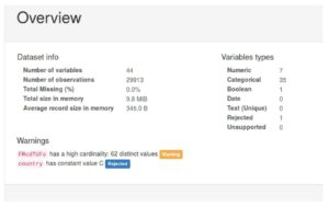
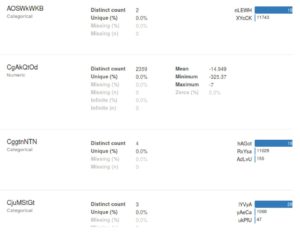
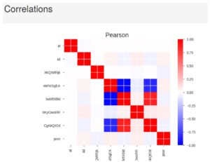
Some more conclusions we can draw are:

1. There seems to be a default value for most categorical fields that is the most common value for the field. (In the above picture, for example, you can see the field AOSWkWKB has a default value it takes 80%+ times)
2. The datasets are highly imbalanced, we need to take care of the fact while training.

Two ways to model the data

If one looks at the datatypes of the objects, they can see that the data is a mix of categorical (attributes which can take one out of a constant number of enumerable values) and numerical values (both floats and integers). In fact, that is how the Random Forest benchmark provided by WorldBank models and is available here. However, when you look at the numerical quantities, they are not that numerous and might represent quantities like Date Of Birth etc. (If you have taken the Coursera course, Dmitry talks about a similar set of fields in handling anonymized datasets section). So another approach we wanted to try was to treat all the fields as categorical attributes. We ended up trying both.

Data Imbalance

Another important property of dataset is the imbalance between +ve and -ve classes (non-poor people vastly outnumber poor people).  For the country A, the data is still balanced, but for B and C, the data has a very skewed distribution. To train models on such skewed data, we tried different approaches using an imbalanced-learn library in Python:

1. Training on the skewed dataset (which worked OK, not too great)
2.  Training on a dataset with negative class undersampled (which performed very badly, even the best Machine Learning models could work just as well as the baseline with this dataset)
3. Oversampling the +ve class (Which worked quite well)
4. Oversampling using SMOTE algorithms (did not work as well as normal oversampling, primarily because SMOTE algorithm is not really defined for categorical attributes)
5. Oversampling using ADASYN (did not work as well as normal oversampling)

Preprocessing

The dataset was preprocessed as follows:

1. All categorical features were converted to binary features.
2. The numerical values were normalized. Both max-min and mean-std normalization were tested.
3. Household level and Individual level data was merged (individual level data had separate data for each member of all household provided).  Only household level data was retained for attributes common in individual and household data. All numerical features in the household were taken a mean of (which might have not been the best way) and all categorical values were aggregated to the oddest value amongst the household (So for example if feature X had value 1,1,1,0 in the household, we would take combined value for the household as 0). The reason is that a lot of categorical variables hold the default value and we expected the odd value to have more information.  

Approaches we tried

We now talk about multiple approaches that we tried.

• First, we talk about things that did not work:

1. We thought that the default attributes for categorical fields might not be useful for modeling. To check this, we trained Machine Learning models both with and without the default attributes. Models not being fed default attributes consistently performed worse than ones being fed the default values.
2. SMOTE and ADASYN oversampling didn't give better results than normal oversampling.
3. Two staged Machine Learning, the first to create a decision tree to get the importance of features and the other to train on most important features. We did not get any gains by trying this technique.
4. Trying different methods to normalize numerical data did not change accuracy. However, non-normalized numerical attributes got worse accuracy.

• The tricks which helped us increase our score:

1. Combination of numerical and categorical feature worked better to train algorithms than all categorical attributes. At least for decision trees.
2. Choice of default values for missing data helped us better our accuracy. We started by making all missing values as Zero, but later used -999 which worked better.
3. Grid Search across Machine Learning hyperparameters got us 2-4% better on the validation set with no effort.
4. A strong AutoML baseline helps us get started well.

• The tricks that we wanted to try but couldn’t/didn’t/were too lazy to code :

1. Feature Engineering by taking cartesian product of non-default categorical values and then choosing important features to train the model on.
2. Feature Engineering by combining numerical features in different ways and doing feature selection on generated features.
3. Trying ensembles of multiple models. We had earlier fixed the goal to get one good model but still ended up training many methods. We could have combined them as an ensemble like stacking.

Machine Learning Algorithms

Libraries we used: SKLearn, XGBOOST, and TPOT

We will now talk about Machine Learning approaches we tried out. Talking about things in a chronological order, as in what order we tried approaches in. Please note that all tricks that worked for us weren’t around since our first try and we included them one by one. Please see the points for each trial to understand what was the pipeline at that time. All Machine Learning models used were from Scikit Learn library unless otherwise stated.

• The usual suspects with default parameters

1. We started with trying out the usual suspects with default parameters. Logistic regression, SVM, and Random Forests. We also tried a new library called CATBOOST, but we couldn’t find a lot of documentation about its hyperparameters nor could fit it well on data, so decided to replace it with the more well-known XGBOOST. We also had knowledge about XGBOOST hyperparameter tuning (which we knew we had to do in later stages).
2. The first attempt modeled all the columns as categorical data and imbalanced dataset.
3. All the models fit ok and give us way better accuracy than coin toss on validation data. That kind of tells us that the data extraction pipeline is OK (that has no obvious bugs but needs to be finetuned more).
4. Like the baseline provided by competition providers, Random Forests and XGBOOST with default hyperparameters show good results.
5. LR and SVM can model the data well (not as well as RF and XGBOOST due to less variance in the default hyperparameters). SVM (SKLearn SVC) had a good accuracy too, but the probabilities it returns are not really usable in SKLearn (which I found is a common issue with default hyperparameters), which made us drop SVM as the competition judged on mean logloss and this would require extra effort to make sure that the probability numbers are right. It's just that probabilities SVC returns are not exactly probability but some type of score.

• TPOT: AutoML makes a good baseline

1. Still continuing with all features being taken as categorical, we tried to fit a baseline using an AutoML method called TPOT.
2. TPOT uses genetic algorithms to figure out a good Machine Learning pipeline for the problem at hand along with what hyperparameters to use with it.
3. This got us in top 100 in the competition public leaderboard at the time we submitted it.
4. TPOT takes time to figure out pipeline and converged in a few hours for the entire dataset.

• Can Neural Networks be used? Neural Networks anyone?

The love we have for Deep Learning made our hands itch to try something Neural Networks-y. We set ahead to train a good Neural Network algorithm that could solve this problem too. Please note at this time, we were doing experiments considering all columns as categorical. What is a problem that has many categorical variables and needs to predict a label? Text Classification. That is one place where Neural Networks shine a lot. However, unlike text,  this dataset has no concept of sequence, so we decided to use a Neural Network common in text classification, but doesn’t take order into account. That algorithm is FastText. We wrote a (deep) version of fast text like the algorithm in keras to train on the dataset. Another thing we did to train Neural Network was oversampling minority class, as it did not train well on imbalanced data.

[caption id="attachment_3089" align="alignnone" width="727"]

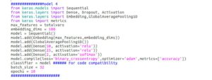
FFNN Used[/caption]

We tried training using the recently proposed Self Normalized Neural Networks. This gave us free bump of accuracy on the validation set.

[caption id="attachment_3090" align="alignnone" width="746"]

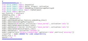
Self Normalized FFNN (SELU) we used[/caption]

Although we get gains in accuracy on validation set when we use Deep Neural Networks, esp. Country B where the highest accuracy we ever received (even better than our best performing model) was using Self Normalized Deep Neural Network, the results don’t translate on the leaderboard where we keep getting low scores (high logloss).

• Towards improving the AutoML Baseline and tuning XGBOOST

AutoML baseline we created still stared us in our face as all our handcrafted methods were still worse. We hence decided to switch to the tried and tested XGBOOST models to better the scores. We wrote a data pipeline for trying out different tricks we have mentioned (successful/unsuccessful) at the start of the segment and a pipeline to Grid Search over different hyperparameters and try a 5-fold Cross-Validation.

[caption id="attachment_3091" align="alignnone" width="739"]

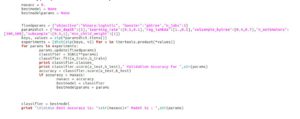
Grid Search Example for the single validation set[/caption]

The tricks which worked above combined with Grid Search gave massive boosts to our scores and we could beat 0.2 logloss and then 0.9 logloss score too. We tried another TPOT AutoML with a dataset generated by our successful tricks, but it could only take up to a pipeline with close to 0.2 logloss on the leaderboard. So ultimately the XGBOOST model turned out to be the best one. We couldn’t get the accuracy of the same order when we tried to Grid Search over parameters of a Random Forest algorithm.

Our score/rank got slightly worse on the private leaderboard as compared to public competition leaderboard. We ended the competition at around 90 percentile.

We hope you liked the article. Please Sign Up for a free Komprehend account to start your AI journey. You can also check demo’s of Komprehend AI APIs here.

‍